Generative adversarial network(GAN) is an awesome technique to generate new data which follows the same distribution as that of training data. I won’t repeat same stuff that you can find on other blogs, this post basically aims to implement an application that uses gans. I will link a post below to learn general gan
Okay, now that you know what a Gan (and DCGan) is and how it works, let’s get ahead with our application. We are going to build a pokemon image generator, how cool is that right? Basically, we will give some random input vector to our model and it will output a whole new pokemon image. We are going to build yet another flavor of GAN called as Wgan (Wasserstein Gan). Before we begin to see the code I’ll quickly explain what WGan is and how is it different than vanilla Gan or DCGan.
WGan
Wgan is just a vanilla Gan but with a better loss function, it uses Wasserstein distance to quantify the difference between generated and the actual image. The primary advantage of this distance is that the model learns in a controlled way, as in the training process is stabilized. I would be going much into the mathematics of distance metric but if someone is interested they can read this amazing post.
So below is the algorithm from the original paper, let’s look at the whole process as we are going to code it.
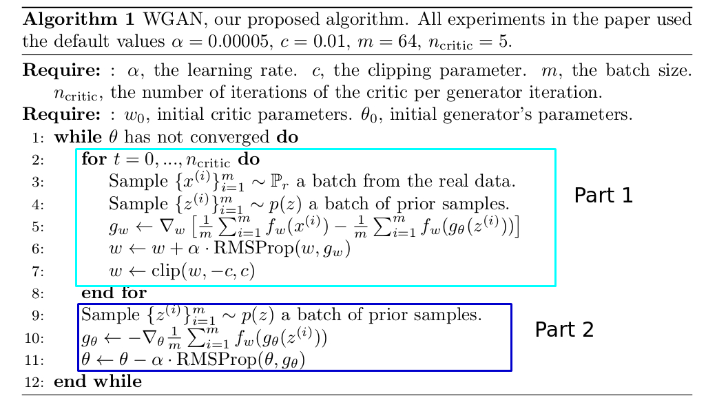
For the 1st part of the algorithm, the discriminator is getting trained, a for loop is there because discriminator should get more training than the generator, this is how the algo flow goes
- Sample a batch from the real data, here basically we will feed a subset of our dataset.
- here we generate a random input of random dimension, of the same batch size as that of real data.
- Here we calculate gradients, by taking the difference between the discriminator output of the real image to that of the fake (generated image). Here the function ‘f’ is for the discriminator and ‘g’ for the generator.
- Then the values of thetas are updated according to the RMS prpo equation.
- Finally we clip the value of thetas, so that the values lie in compact space.
The second part is quite easy to understand, as the gradients values are calculated as the negative of the output generated by the discriminator for the fake images.
Enough of theory already! Let’s build the application
Application
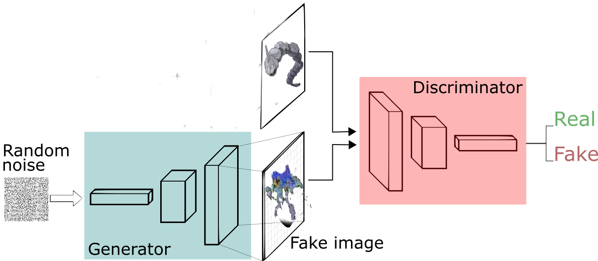
Let’s first talk about the whole architecture and then as we proceed further, other parts will be revealed along with the code. Below is the whole architecture, first we feed some random input of random dimension the generator which then gives a fake image. This fake image is fed to the discriminator along with the real image, using it’s output the discriminator and the generator both get trained and over time real looking images are produced.
This is how the code structured is followed
Before we begin the code for this project can be cloned from this repo.
Let’s start coding
Data Preprocessing
First, have a look at the dataset, the dataset consists of total 819 pokemons of dimension 128x128, which were then augmented to make a dataset of size 8190. You can download the original dataset from here. Below are some of the images from the dataset.
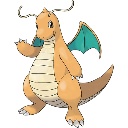
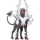
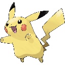
Dragonite Mega Houndoom Pikachu
The code for augmentation is written in augment.py, I won’t go through the whole code but will just mention the crux of it, and the rest is self-explanatory.
augment.py
from PIL import Image
import os


#flips single image
def flip_image(image):
    new_img = image.transpose(Image.FLIP_LEFT_RIGHT)
    return new_img

# rotates single image
def rotate_image(image, degree):
    new_img = image.convert('RGBA') # convert to RGBA to get transparent background
    new_img = new_img.rotate(degree) #rotate the image by the specified degree
    background = Image.new("RGB", new_img.size, (255, 255, 255))
    background.paste(new_img, mask=new_img.split()[3]) # 3 is the alpha channel
    return background
Next we are going to read the augmented dataset, normalize it and then save it in numpy format for ease of use.
preprocess.py
import numpy as np
import os
import tensorflow as tf


CHANNEL = 3 # channels
size = [128,128]  # WxH
DATA_FILE = 'data/augmented' #read the data from this folder
SAVE_FILE = 'dataPokemonAugmented.npy'

current_dir = os.getcwd()
pokemon_dir = os.path.join(current_dir, DATA_FILE)
images = []
# append the address of all the images in the list
for each in os.listdir(pokemon_dir):
    images.append(os.path.join(pokemon_dir,each))

decoded_files = []
sess = tf.Session()


for im in images:
    content = tf.read_file(im)
    #decode all the images in jpeg format
    img = tf.image.decode_jpeg(content, channels = CHANNEL)
    decoded_files.append(img)

X = []
# normalize 1000 at a time
for i in range(0,len(decoded_files),1000):

    #resize the images and the convert it in between 0 to 1
    img = tf.to_float(tf.image.resize_images(decoded_files[i:i+1000], size, method=tf.image.ResizeMethod.BICUBIC)) / 127.5 - 1
    img =  sess.run(img)
    for j in img:
        j = cv2.cvtColor(j, cv2.COLOR_BGR2RGB) # we need to convert to RGB since tf reads in BGR and when you save the generated images you will need RGB.
        X.append(j)

np.savez(open(SAVE_FILE,'w'),X=X) #save the image in the numpy format
Generator
Generator’s task is to generate a new image from a random input of random dimension, basically a generator is just a standard de-convolutional layer. Below is the structure of the network, assume the series of operations for 1 data point.
| Name | Input Dimension | Output Dimension |
|---|---|---|
| Fully connected | random_dimension | 2048 (44128 (WxHxC, random numbers)) |
| reshape | 2048 | 4x4x128 |
| conv2d transpose 1 | 4x4x128 | 8x8x64 |
| conv2d transpose 2 | 8x8x64 | 16x16x32 |
| conv2d transpose 3 | 16x16x32 | 64x64x8 |
| conv2d transpose 4 | 64x64x8 | 128x128x3 |
Of-course every conv2d transpose layer is followed by activation and also batch normalization is added for stability.
Let’s look at the code for generator
def generator(input, random_dim, is_train, reuse=False):
  c4, c8, c16, c32, c64 = 128, 64, 32, 16,8  # kernels in respective layers
  s4 = 4 # just a random start value
  output_dim = 3  # channel of the image
  with tf.variable_scope('gen') as scope:
      if reuse: # we need to reuse the variables as we will call this function multiple times
          scope.reuse_variables()

      #fully connected layer
      w1 = tf.get_variable('w1', shape=[random_dim, c4 * s4 * s4], dtype=tf.float32,
                           initializer=tf.truncated_normal_initializer(stddev=0.02))
      b1 = tf.get_variable('b1', shape=[c4 * s4 * s4], dtype=tf.float32,
                           initializer=tf.constant_initializer(0.0))

      flat_conv1 = tf.add(tf.matmul(input, w1), b1, name='flat_conv1')

      # 1st conv transpose box
      # 4*4*256
      conv1 = tf.reshape(flat_conv1, shape=[-1, s4, s4, c4], name='conv1')
      bn1 = tf.contrib.layers.batch_norm(conv1, scope='bn1', is_training=is_train, epsilon=1e-5, decay = 0.9, updates_collections=None)
      act1 = tf.nn.relu(bn1, name='act1')

      #2nd conv box
      # 8*8*64
      conv2 = tf.layers.conv2d_transpose(act1, c8, kernel_size=[5, 5], strides=[2, 2], padding="SAME",
                                         kernel_initializer=tf.truncated_normal_initializer(stddev=0.02),
                                         name='conv2')
      bn2 = tf.contrib.layers.batch_norm(conv2, scope='bn2', is_training=is_train, epsilon=1e-5, decay = 0.9, updates_collections=None)
      act2 = tf.nn.relu(bn2, name='act2')

      #3rd conv box
      # 16*16*32
      conv3 = tf.layers.conv2d_transpose(act2, c16, kernel_size=[5, 5], strides=[2, 2], padding="SAME",
                                         kernel_initializer=tf.truncated_normal_initializer(stddev=0.02),
                                         name='conv3')
      bn3 = tf.contrib.layers.batch_norm(conv3, scope='bn3', is_training=is_train, epsilon=1e-5, decay = 0.9, updates_collections=None)
      act3 = tf.nn.relu(bn3, name='act3')

      #fourth conv box
      # 32*32*16
      conv4 = tf.layers.conv2d_transpose(act3, c32, kernel_size=[5, 5], strides=[2, 2], padding="SAME",
                                         kernel_initializer=tf.truncated_normal_initializer(stddev=0.02),
                                         name='conv4')
      bn4 = tf.contrib.layers.batch_norm(conv4, scope='bn4', is_training=is_train, epsilon=1e-5, decay = 0.9, updates_collections=None)
      act4 = tf.nn.relu(bn4, name='act4')


      #fifth conv box
      # 64*64*8
      conv5 = tf.layers.conv2d_transpose(act4, c64, kernel_size=[5, 5], strides=[2, 2], padding="SAME",
                                                 kernel_initializer=tf.truncated_normal_initializer(stddev=0.02),
                                                 name='conv5')
      bn5 = tf.contrib.layers.batch_norm(conv5, scope='bn5', is_training=is_train, epsilon=1e-5, decay = 0.9, updates_collections=None)
      act5 = tf.nn.relu(bn5, name='act5')

      #output
      # 128*128*3
      conv6 = tf.layers.conv2d_transpose(act5, output_dim, kernel_size=[5, 5], strides=[2, 2], padding="SAME",
                                         kernel_initializer=tf.truncated_normal_initializer(stddev=0.02),
                                         name='conv6')

      act6 = tf.nn.tanh(conv6, name='act6')

      return act6
The above function will return an activation operation which will basically our generated image.
Discriminator
The task of discriminator is to get the difference between original image and the generated image, it is a basic convolutional neural network, but the activation function is different. Instead of normal relu we will be using leaky relu. The architecture of the Discriminator is same as generator but in reverse diagram, below is the table illustrating the architecture.
| Name | Input Dimension | Output Dimension |
|---|---|---|
| conv 1 | 128x128x3 | 64x64x16 |
| conv 2 | 64x64x16 | 32x32x32 |
| conv 3 | 32x32x32 | 16x16x64 |
| conv 4 | 16x16x64 | 8x8x128 |
| fully connected | 8x8x128 | 1 |
# leaky relu function
def lrelu(x, leak=0.3, n="lrelu"):
    with tf.variable_scope(n):
        f1 = 0.5 * (1 + leak)
        f2 = 0.5 * (1 - leak)
        return f1 * x + f2 * abs(x)

def discriminator(input, is_train, reuse=False):
    c2, c4, c8, c16 = 16, 32, 64, 128  # number of kernels respectively
    with tf.variable_scope('disc') as scope:
        if reuse:
            scope.reuse_variables()

        #1st conv box
        # 64x6416
        conv1 = tf.layers.conv2d(input, c2, kernel_size=[5,5], strides=[2, 2], padding="SAME",
                                 kernel_initializer=tf.truncated_normal_initializer(stddev=0.02),
                                 name='conv1')
        act1 = lrelu(conv1, n='act1')

        #2nd conv box
        # 32x32x32
        conv2 = tf.layers.conv2d(act1, c4, kernel_size=[5,5], strides=[2, 2], padding="SAME",
                                 kernel_initializer=tf.truncated_normal_initializer(stddev=0.02),
                                 name='conv2')
        bn2 = tf.contrib.layers.batch_norm(conv2, scope='bn2', is_training=is_train, epsilon=1e-5, decay = 0.9, updates_collections=None)
        act2 = lrelu(bn2, n='act2')

        #3rd conv box
        # 16x16x64
        conv3 = tf.layers.conv2d(act2, c8, kernel_size=[5,5], strides=[2, 2], padding="SAME",
                                 kernel_initializer=tf.truncated_normal_initializer(stddev=0.02),
                                 name='conv3')
        bn3 = tf.contrib.layers.batch_norm(conv3, scope='bn3', is_training=is_train, epsilon=1e-5, decay = 0.9, updates_collections=None)
        act3 = lrelu(bn3, n='act3')

        #4th conv box
        # 8x8x128
        conv4 = tf.layers.conv2d(act3, c16, kernel_size=[5,5], strides=[2, 2], padding="SAME",
                                 kernel_initializer=tf.truncated_normal_initializer(stddev=0.02),
                                 name='conv4')
        bn4 = tf.contrib.layers.batch_norm(conv4, scope='bn4', is_training=is_train, epsilon=1e-5, decay = 0.9, updates_collections=None)
        act4 = lrelu(bn4, n='act4')

        shape = act4.get_shape().as_list()
        dim = shape[1] * shape[2] * shape[3]

        #fully connected (just a single value)
        fc1 = tf.reshape(act4, shape=[-1, dim], name='fc1')
        w1 = tf.get_variable('w1', shape=[fc1.shape[1], 1], dtype=tf.float32,
                             initializer=tf.truncated_normal_initializer(stddev=0.02))
        b1 = tf.get_variable('b1', shape=[1], dtype=tf.float32,
                             initializer=tf.constant_initializer(0.0))

        # in wgan we don't use activation in the last layer
        output = tf.add(tf.matmul(fc1, w1), b1, name='output')
        return output
The discriminator just returns a single value in the end so that we can compare the two outputs directly, also note that we don’t apply any activation function for the output as it will hide the actual estimate and disturb the learning.
Train
Before we write our train function, I will just write some utility functions.
Get Next Batch
def getNextBatch(X,pos,BATCH_SIZE):
    if pos+BATCH_SIZE > len(X):
        np.random.shuffle(X)
        pos = 0

    return X[pos:pos+BATCH_SIZE], pos+BATCH_SIZE
This function will just return a new batch of data, the size of which is specified by ‘BATCH_SIZE’. ‘pos’ is the current position in the dataset ‘X’, the variable ‘pos’ is maintained in the train function.
Save generated images
def imwrite(image, path):
  image = (image * 255.).astype(dtype=np.int16) % 256 # get it the range 0-255
  scipy.misc.imsave(path, image) #save the image
Now, let’s write our train function, comments in the below code will be enough for the explanation.
First, let’s just define our parameters and placeholders
def train():

  ## let's read the saved file
  save_file = open("dataPokemonAugmented.npy",'r')
  X = np.load(save_file)["X"]

  #Parameters

  d_iters = 5 # the number of iteration for discriminator per interation of generator
  HEIGHT, WIDTH, CHANNEL = 128,128,3
  BATCH_SIZE = 64
  EPOCHS = 1000
  random_dim = 100
  learning_rate = 2e-4
  pos = 0  #current position in the dataset
  total_batch = 0 #total batches done
  generate_noise = np.random.uniform(-1.0,1.0,size=[BATCH_SIZE, random_dim]).astype(np.float32) #noise to generate new pokemons during the training process
  MODEL_ADD = 'models/pokemonModelV1/' #address to save the trained model


  #placeholder to feed the value to our network
  is_train = tf.placeholder(tf.bool, name='is_train')
  real_image = tf.placeholder(dtype=tf.float32,shape=[None,HEIGHT,WIDTH,CHANNEL],name='image_input') # to feed real image
  random_inp = tf.placeholder(dtype=tf.float32,shape=[None,random_dim],name='random_inp')
Next we will define our graph operations.
  #generator operations
  fake_image_generator = generator(random_inp, random_dim,is_train, reuse=False)
  sample_img = generator(random_inp,random_dim,is_train,reuse=True) #this operation is just defined to generate sample images during training

  #discriminator operations
  real_result = discriminator(real_image,is_train)
  fake_result = discriminator(fake_image_generator,is_train,reuse=True)
Now since we have defined our operations our next step is to define loss functions for discriminator and generator and set up optimizers.
  #disc and genr loss according to the Wgan paper
  d_loss = tf.reduce_mean(fake_result)- tf.reduce_mean(real_result)
  g_loss =  -tf.reduce_mean(fake_result)

  # get all the trainable variables i.e variables that are going to be optimized
  t_vars = tf.trainable_variables()
  d_vars = [var for var in t_vars if 'disc' in var.name]
  g_vars = [var for var in t_vars if 'gen' in var.name]

  # setup rmmprop optimizers
  trainer_d = tf.train.RMSPropOptimizer(learning_rate=learning_rate).minimize(d_loss, var_list=d_vars)
  trainer_g = tf.train.RMSPropOptimizer(learning_rate=learning_rate).minimize(g_loss, var_list=g_vars)

  # clip operation to clip the value of thetas, according to the paper
  d_clip = [v.assign(tf.clip_by_value(v, -0.01,0.01)) for v in d_vars]
Next we will write the core of the function, the training loop
  init = tf.global_variables_initializer() #initialize all the variables
  saver = tf.train.Saver(max_to_keep=4) #saver object to save our trained models.
  sess = tf.Session()
  sess.run(init)

  for epoch in range(EPOCHS):

      # split the data into batches
      for batch in range(X.shape[0]/BATCH_SIZE):
          d_iters = 5

          #this if condition is for training disc more number of times, occasionally.
          if total_batch%500==0 or total_batch < 25:
              d_iters = 25


          ## discriminator loop
          for d_n in range(d_iters):
              curr_batch, pos = getNextBatch(X,pos,BATCH_SIZE) #get a batch of data
              train_noise = np.random.uniform(-1.0,1.0,size=[BATCH_SIZE, random_dim]).astype(np.float32) #random noise to feed to generator
              sess.run(d_clip)
              _, dLoss = sess.run([trainer_d, d_loss], feed_dict={real_image:curr_batch,random_inp:train_noise,is_train:True})

          #train the generator
          train_noise = np.random.uniform(-1.0,1.0,size=[BATCH_SIZE, random_dim]).astype(np.float32)
          _, gLoss = sess.run([trainer_g, g_loss], feed_dict={random_inp:train_noise,real_image:curr_batch,is_train:True})

          total_batch += 1

      #print loss every 5th epoch
      if epoch%5==0:
          select = np.random.randint(0,X.shape[0],BATCH_SIZE) # take some random points to run the network on
          curr_batch = X[select]
          train_noise = np.random.uniform(-1.0,1.0,size=[BATCH_SIZE, random_dim]).astype(np.float32)
          dLoss = sess.run(d_loss, feed_dict={real_image:curr_batch,random_inp:train_noise,is_train:True}) # get the disc loss

          train_noise = np.random.uniform(-1.0,1.0,size=[BATCH_SIZE, random_dim]).astype(np.float32)
          gLoss = sess.run(g_loss,feed_dict={random_inp:train_noise,is_train:True}) #generator loss
          print "EPOCH: "+str(epoch)+" Disc Loss: "+str(dLoss)+" Gen Loss: "+str(gLoss) #print

      #save some generated images and the trained model every 40th epoch
      if(epoch%40==0):
          saver.save(sess,MODEL_ADD+'model', global_step=epoch, write_meta_graph=False)

          #generate images
          os.makedirs('generated/'+str(epoch)+'/') # make directory for that epoch
          gen_images = sess.run(sample_img,feed_dict={random_inp:generate_noise,is_train:False})
          #write images
          for g in range(len(gen_images)):
              imwrite(gen_images[g],'generated/'+str(epoch)+"/"+str(g)+'.jpg')
That’s it for the training loop, now you can run the code and the model will start training.
I have uploaded the training process and the loss function graph on my github repo.
Results
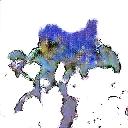
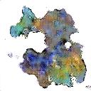
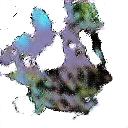
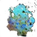
Below are some of the generated images, although they are not that precise and real looking, but the model at least learned the pattern in these pokemons.
These were generated after 1000 epochs
Conclusion
In this post, I talked about Wgans to generate new pokemon images. Links to learn general Gan and DcGan were attached in the introduction section, and then the core algorithm of WGan was explained. Finally, we went through the code which was in tensorflow. The results were not that mesmerizing but the model learned the pattern of the data, with greater amount of data and relatively awesome compute power Wgans are capable of generating real looking images. If you have any doubts, please ask in the comments section and don’t forget to star/fork the repository for this application and also don’t forget to share the post.
Thankyou, until next time.